Austin Silveria, Soham Govande, Dan Fu | Star on GitHub

In Part I, we introduced Chipmunk, a method for accelerating diffusion transformers by dynamically computing sparse deltas from cached activations. Specifically, we showed how exploiting the slow-changing, sparse nature of diffusion transformer activations can dramatically reduce computational overhead, yielding substantial speedups in both video and image generation tasks.

Part II shifts focus to building deeper theoretical intuition behind why dynamic column-sparse deltas are effective. We’ll explore the following key areas:

1. Latent Space Dynamics: Understanding diffusion transformers as performing iterative “movements” through latent space.

2. Momentum in Activations: How these latent-space movements demonstrate a form of “momentum,” changing slowly across steps.

3. Granular Sparsity: Why sparsity at the level of individual attention and MLP vectors effectively captures cross-step changes.

4. Efficient Computation: Techniques for aligning sparsity patterns with GPU hardware constraints, achieving practical speedups.

Let’s dive deeper and unpack the theoretical foundations of Chipmunk’s dynamic sparsity!

DiTs: Paths Through Latent Space

Few-step models, step distillation, and training-free caching have all significantly accelerated diffusion inference. Where do these lines of research converge? We’re interested in conceptually unifying these approaches and understanding the role of sparsity and caching at a more granular level—within individual attention and MLP operations. This post will focus on two things: developing a conceptual framework for thinking about diffusion efficiency and designing hardware-efficient sparse caching algorithms for attention and MLP.

When a Diffusion Transformer (DiT) generates content, it moves from a random noise point to a coherent output point. The concrete representation denoised by the DiT is the same as language models: A set of tokens, each represented by a high-dimensional vector. In each denoising step, the DiT takes this representation as input and computes a residual using nearly the same architecture as a normal Transformer – the notable differences include using full self-attention (though some methods use causal) and applying element-wise scales and shifts (modulations) to activations as a function of timestep and static prompt embeddings.

The simplest generation path in latent space would be a straight line. One big step from noise to output–one forward pass through the DiT to compute a single residual of the per-token latent vectors.

This is the ideal of rectified flow and consistency models. Use a single inference step to jump directly to the output point from anywhere in space.

But what makes sequential, multi-step inference expressive is the ability for it to update its trajectory at each step. Later forward passes of the DiT get to compute their outputs (movements in latent space) as a function of the prior steps’ outputs.

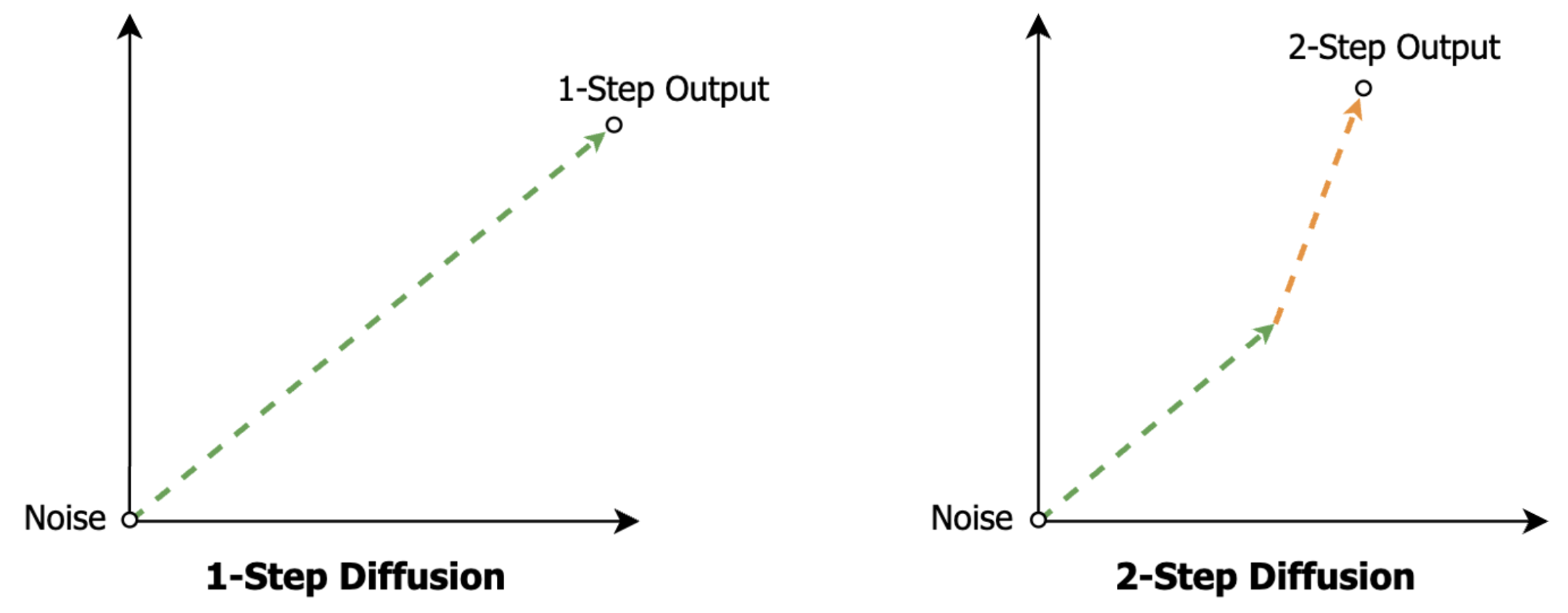
Even with rectified flow and consistency model training, we are still finding that multiple sequential steps of these models improve quality at the cost of longer generation times. This observation seems quite fundamental, like a reasoning model taking more autoregressive steps to solve a difficult problem.

So how can we move towards generation with the efficiency of a single step and the expressiveness of multiple steps?

Caching + sparsity is one possible path. We’ll see that per-step DiT outputs, or movements in latent space, change slowly across steps, allowing us to reuse movements from earlier steps. And by understanding the most atomic units of DiT latent space movement, we’ll see that most of this cross-step change can be captured with very sparse approximations.

Latent Space Path Decompositions

So, now we’ve conceptualized DiTs as computing “paths” in latent space, where per-token latent vectors accumulate “movements” in latent space on each step.

But what makes up these per-step latent space movements produced by the DiT?

To get to the root, we’ll make two conceptual moves about what happens in a DiT forward pass:

1. **Attention and MLP are both query, key, value operations.
2. Transformer activations accumulate sums of weighted values from attention and MLP across layers and steps (the “residual stream” interpretation).

Let’s start with the attention and MLP equations:

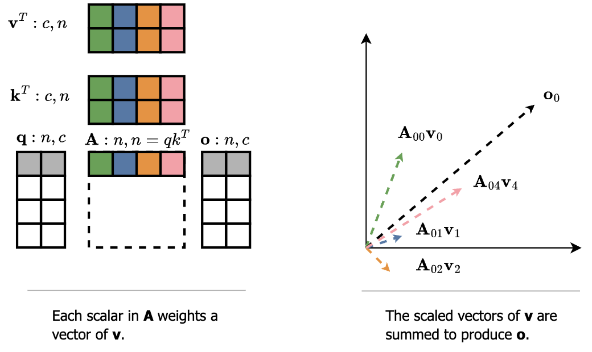
1. Attention: softmax(Q @ KT) @ V
2. MLP: gelu(X @ W1) @ W2

Both operations use a non-linearity to compute the scalar coefficients for a linear combination of value vectors. In attention, the value vectors are dynamic (V is projected from the current token representation). In MLP, the value vectors are static (rows of the weights W2). Thus, in attention, our outputs are a sum of scaled rows in the V matrix, and in MLP, our outputs are a sum of scaled rows in the W2 matrix (the bias is one extra static vector). We can visualize these individual vectors as being summed to produce the total operation output.

To continue decomposing the per-step latent space movements produced by the DiT, we now want to show that these individual vectors are the only components of those larger movements.

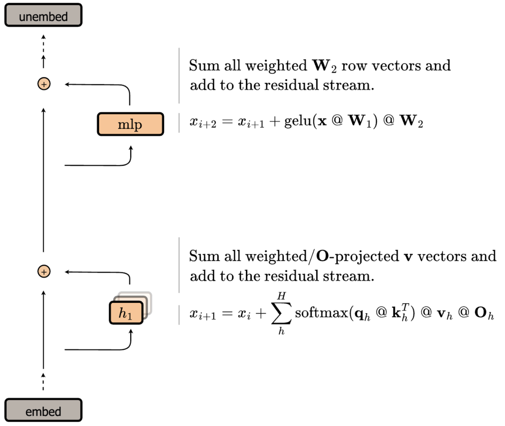
The “residual stream” interpretation of Transformers conceptualizes the model as having a single activation stream that is “read” from and “written” to by attention and MLP operations. Multi-Head Attention reads the current state of the stream, computes attention independently per head, and writes the sum back to the stream as a residual. MLP reads from the stream and adds its output back as a residual.

We now have two observations:

1. Attention and MLP both output a sum of scaled vectors
2. Attention and MLP are the only operations that write to the residual stream

Thus, these individual scaled vectors are the only pieces of information ever “written” to the residual stream, and they all sum together to make larger movements in latent space. Reasoning at the level of these individual vectors will help us do three things:

1. See redundancy in DiT computation at different hierarchical levels (e.g., per-vector/layer/step)
2. Reformulate sparse attention/MLP to selectively recompute fast-changing vectors across steps
3. Map this reformulation to a hardware-efficient implementation

Latent Space Momentum: Some DiT Activations Change Slowly Across Steps

Ok, let’s briefly take stock. We’ve cast DiTs as computing paths in latent space from noise to output over the course of multiple steps, where each step adds a movement (output residual) that affects the movements computed by later steps. We’ve also seen that we can decompose these paths into more atomic units of movement: the scaled vectors output by attention and MLP.

Now to the fun part: What does it mean that some of these movements change slowly across steps? And how can that translate into faster generation?

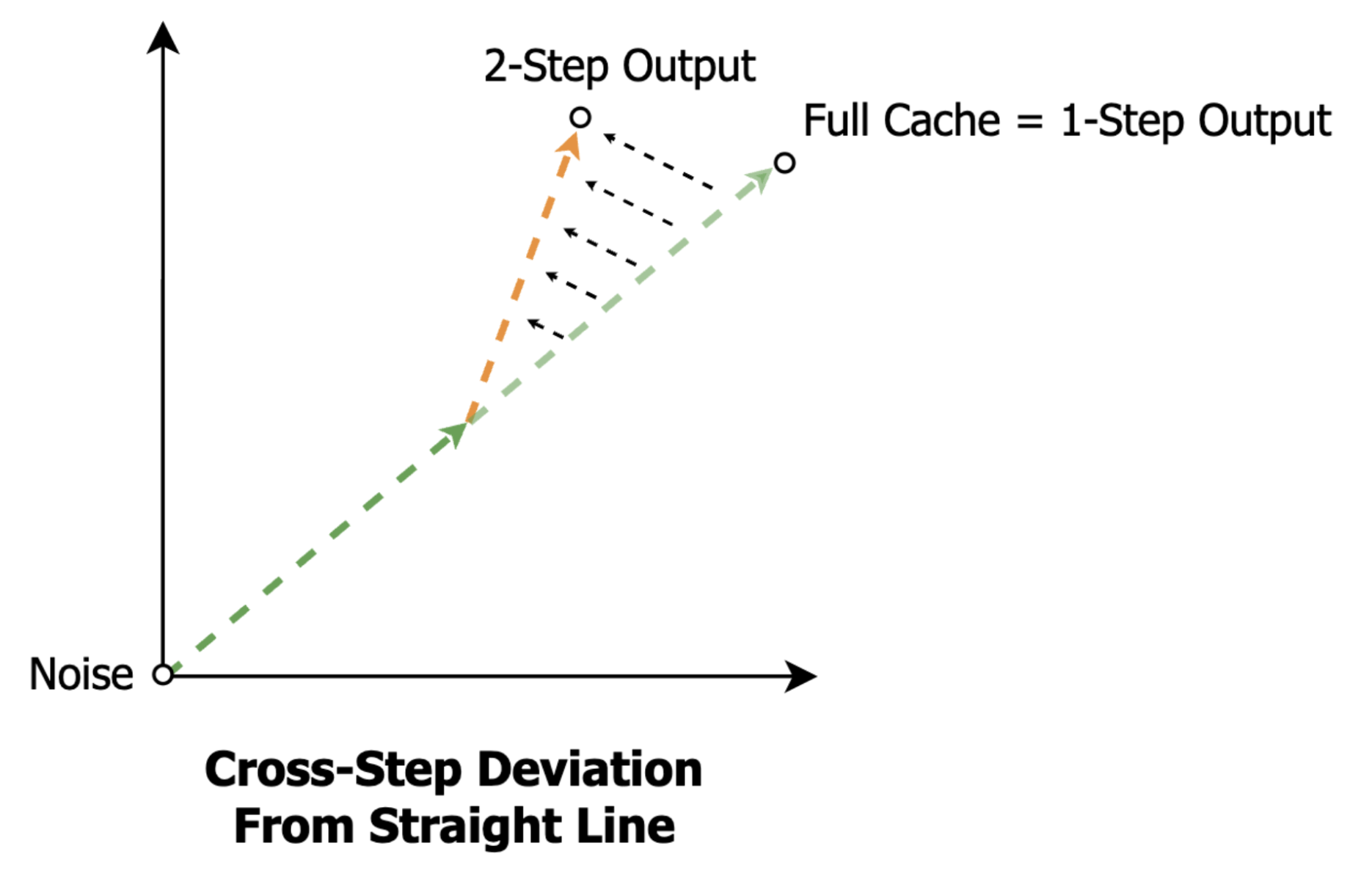
Many works have observed slow-changing activations in DiTs across steps (e.g., full step outputs or per-layer outputs that are similar to previous steps). Translating this into our language, slow-changing activations say that the movements produced in step n are almost the same as the movements produced in step n+1, implying a notion of “momentum” in the movements across steps.

But wait, doesn’t this just mean we’re moving in a near straight line in latent space? Can’t we just use fewer steps then?

The difference comes down to whether all movements change slowly across steps or only a content-dependent subset of movements change slowly across steps. Existing works have observed the latter (e.g., some text prompts result in faster changes in activations (movements) across steps and some tokens exhibit faster changing activations (movements) than others).

Thus, caching methods speed up generation by dynamically identifying and reusing slow-changing movements from previous steps, at the per-step, per-layer, or per-token granularity. Comparing the different hierarchical levels:

1. Step caching reuses the sum of all atomic movements in a previous step for all tokens
2. Layer caching reuses the sum of all atomic movements in a previous layer for all tokens
3. Token caching reuses the sum of all atomic movements in a previous layer for specific tokens

Step distillation, on the other hand, statically allocates fewer steps to all tokens and layers. But, it learns how to do this in a fine-tuning stage, whereas dynamic activation caching methods are currently training-free.

The takeaway here is that we can see step distillation and dynamic activation caching as doing conceptually the same thing: allocating fewer sequential steps to atomic movements in latent space. But, step distillation learns to uniformly allocate fewer steps across all movements, whereas activation caching computes heuristics to non-uniformly allocate fewer steps across all movements.

The intersection will replace those heuristics with gradient descent. And for the best quality-per-FLOP tradeoff, we want to dynamically allocate those steps across all movements with the finest granularity. In the next section, we’ll look at this granular allocation: Identifying the redundancy in cross-step movements at the individual vector level, and reformulating sparse attention and MLP to exploit it.

Latent Subspace Momentum: Sparse Attention/MLP Deltas

We’ve seen that DiT activation caching dynamically allocates fewer steps to slow-changing activation vectors (summed movements in latent space) at varying hierarchical levels (e.g., per-step, per-layer, per-token). Our goal now is to take the granularity of that dynamic allocation to the limit: How can we dynamically allocate fewer steps to specific atomic movements output by attention and MLP? What does this look like in concrete computation?

We’ll make four moves:

1. Attention and MLP step-deltas subtract the old scaled output vectors and add the new scaled output vectors.
2. Sparse intermediate activations compute a subset of the individual output vectors.
3. Attention and MLP are known to be naturally sparse.
4. Attention and MLP step-deltas are even sparser.

To ground ourselves, let’s start with a visualization and concrete computational definition of attention and MLP step deltas. As we saw earlier, attention and MLP both output a sum of scaled vectors, or movements in latent space. Thus, given an attention/MLP output cache, an equivalent definition of a normal dense forward pass on step n is the following: Subtract all of step n-1’s output vectors from the cache, and add all of step n’s new vectors.

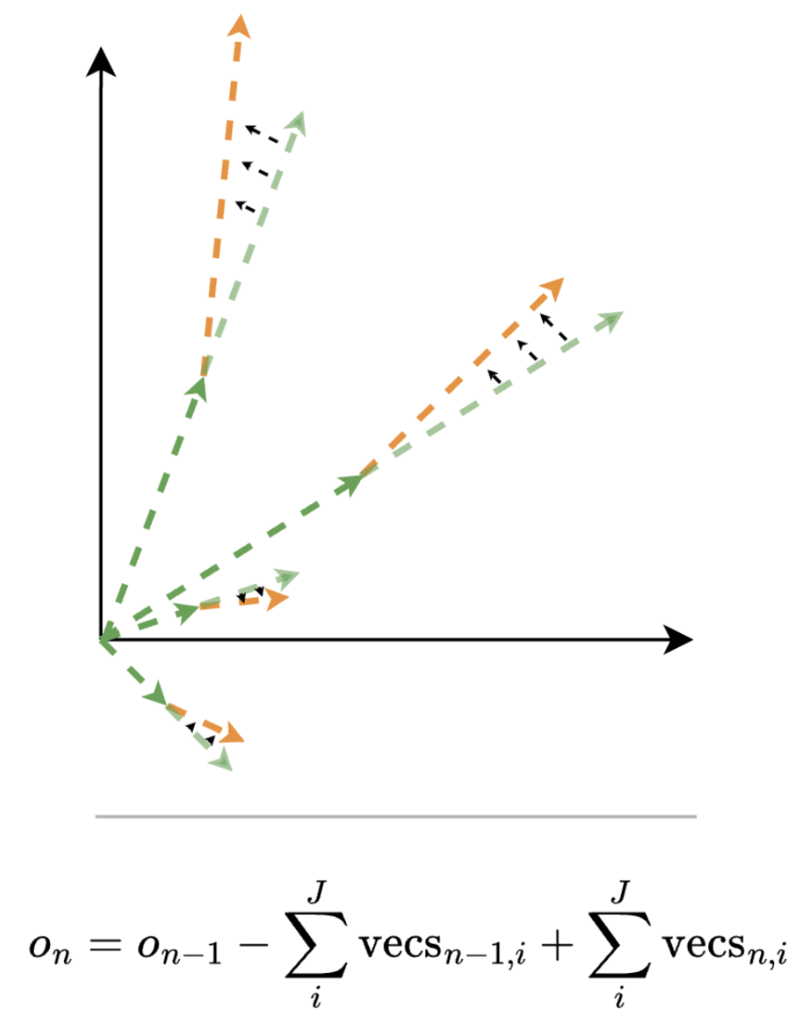
So, replacing all movements in latent space on every step is equivalent to running each step with the normal dense DiT forward pass. But what we would like to do is dynamically replace a subset of these movements on each step. What does this look like in the concrete computation of attention and MLP?

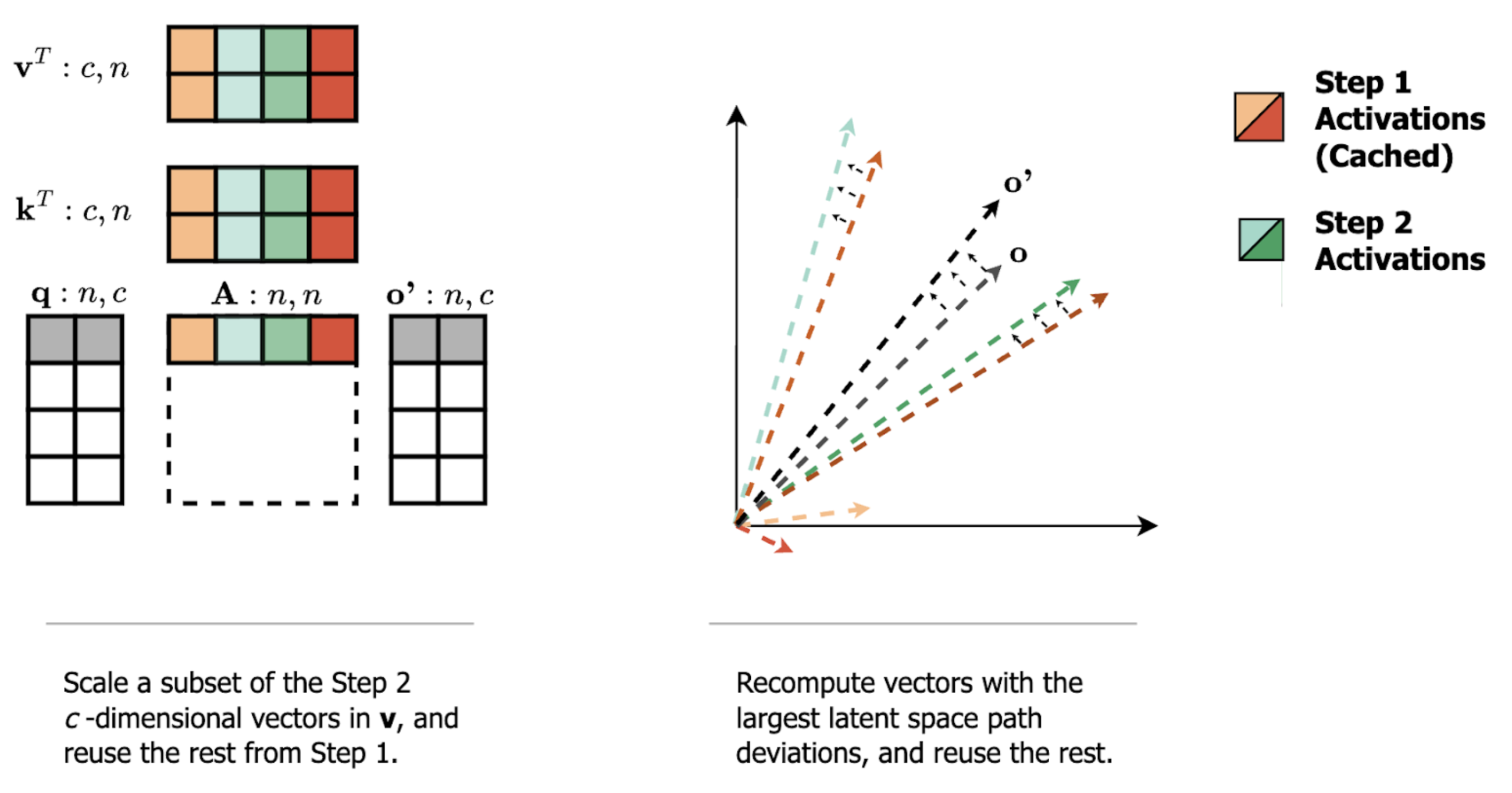
Recall that each value-vector in attention/MLP is scaled by a single scalar value in the intermediate activation matrix. This means that sparsity on the intermediate activation matrix corresponds to removing atomic vector movements from the output. But, if we instead reuse those skipped atomic vector movements from a previous step, we have replaced a subset of the atomic vector movements (i.e., we have computed the sparse step-delta).

But why should we expect the sparse replacement of atomic vector movements across steps (the sparse delta) to be a good approximation of the total cross-step change in the attention/MLP’s output?

We can combine the previously mentioned observation of slow-changing activations with another known observation: Attention and MLP intermediate activations are naturally sparse. In attention, it is common to see queries place a very large percentage of their attention probability mass on a small subset of keys–this means that the output will mostly be made up of the small subset of associated rows of V. And in MLP, previous works have observed significant sparsity in the intermediate activations of both ReLU and GeLU-based layers, meaning that the output will mostly be made up of the top activated rows of W2.

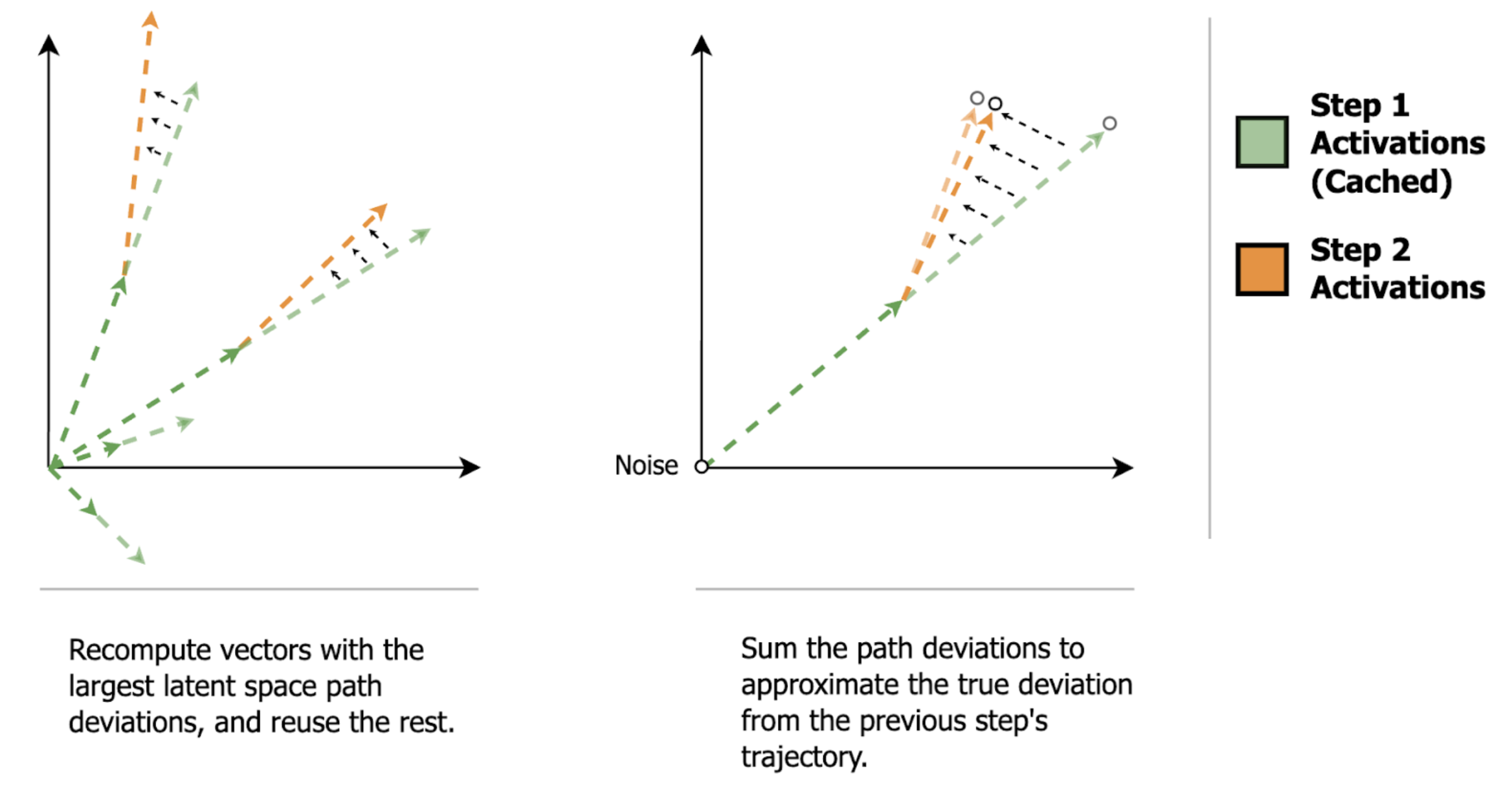
Putting these two observations together, we should expect to be able to capture most of the cross-step change in attention/MLP outputs (step-delta) by replacing the small subset of scaled vectors that change the most. That is, we should be able to capture most of the cross-step path deviation by replacing the atomic movements that change the most.

As an analogy to low-rank approximations, we can think of this like a truncated singular value decomposition, where with a heavy-tailed singular value decomposition, we can get a good approximation of the transformation with only a few of the top singular values. In our case, we can get a good approximation of the cross-step output deltas because the distribution of the intermediate activations is very heavy-tailed.

There is also one fun implication of MLP value-vectors being static vs. attention value-vectors being dynamic. Since the MLP value vectors are rows of the static weight matrix W2, the computation of cross-step deltas can be computed in one shot (instead of subtracting an old set of vectors and adding the new set). Suppose we cache the MLP’s post-nonlinearity activations and output. To replace a subset of the scaled output vectors (atomic movements) on the next step, we can (1) compute the delta of our sparse activations and the cache, (2) multiply this sparse delta with the value-vectors (rows of W2), and (3) add this output directly to the output cache.

Stepping back, the key takeaway from our discussion of sparse deltas is that sparsity on the intermediate activations of attention/MLP can be used to compute a sparse replacement of atomic movements in latent space. Because DiT activations change slowly across steps and attention/MLP are already naturally sparse, we can reuse most of the atomic latent space movements from the previous step and compute a sparse replacement of only the fastest changing movements. But efficiently computing sparse matrix multiplications on GPUs is notoriously difficult, so how can we get this level of granularity while remaining performant?

Tile Packing: Efficient Column Sparse Attention and MLP

In previous sections, we’ve seen that attention and MLP both output a sum of scaled vectors, and that sparsity on the intermediate activations corresponds to only computing a subset of those scaled vectors. The challenge we face now is efficiently computing this sparsity on GPUs, which only reach peak performance with large, dense block matrix multiplications. We’ll briefly summarize the approach of our column-sparse kernel here–see Part II of this post for the details.

The sparsity pattern we’ve been describing thus far, recomputing individual scaled output vectors (atomic latent space movements) for each token, corresponds to [1, 1] unstructured sparsity on the intermediate activations. GPUs do not like this. What they do like is computing large blocks at once, in the size ballpark of [128, 256] (in the current generation). This corresponds to 128 contiguous tokens and 256 contiguous keys/values.

Computing with block sparsity that aligns with the native tile sizes of the kernel is essentially free because the GPU is using the same large matrix multiplication sizes and skips full blocks of work.

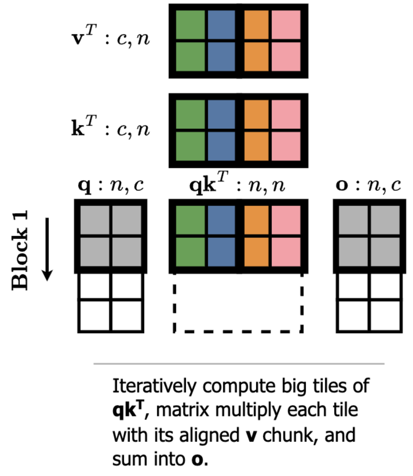
However, there is one optimization we can make to efficiently get to [128, 1] column sparsity. Looking at our matrix multiplication diagram, let’s think through what happens if we reorder the columns of kT and vT. A reordering of kT will apply the same reordering to the columns of A = q @ kT. And if we apply the same reordering to vT, then the end result o is actually the same because the columns of A still align with the correct columns of vT.

What this allows us to do is compute attention or MLP with any ordering of the keys/values in shared memory–thus we can pack our sparse keys/values from non-contiguous rows in global memory into a dense tile in shared memory.

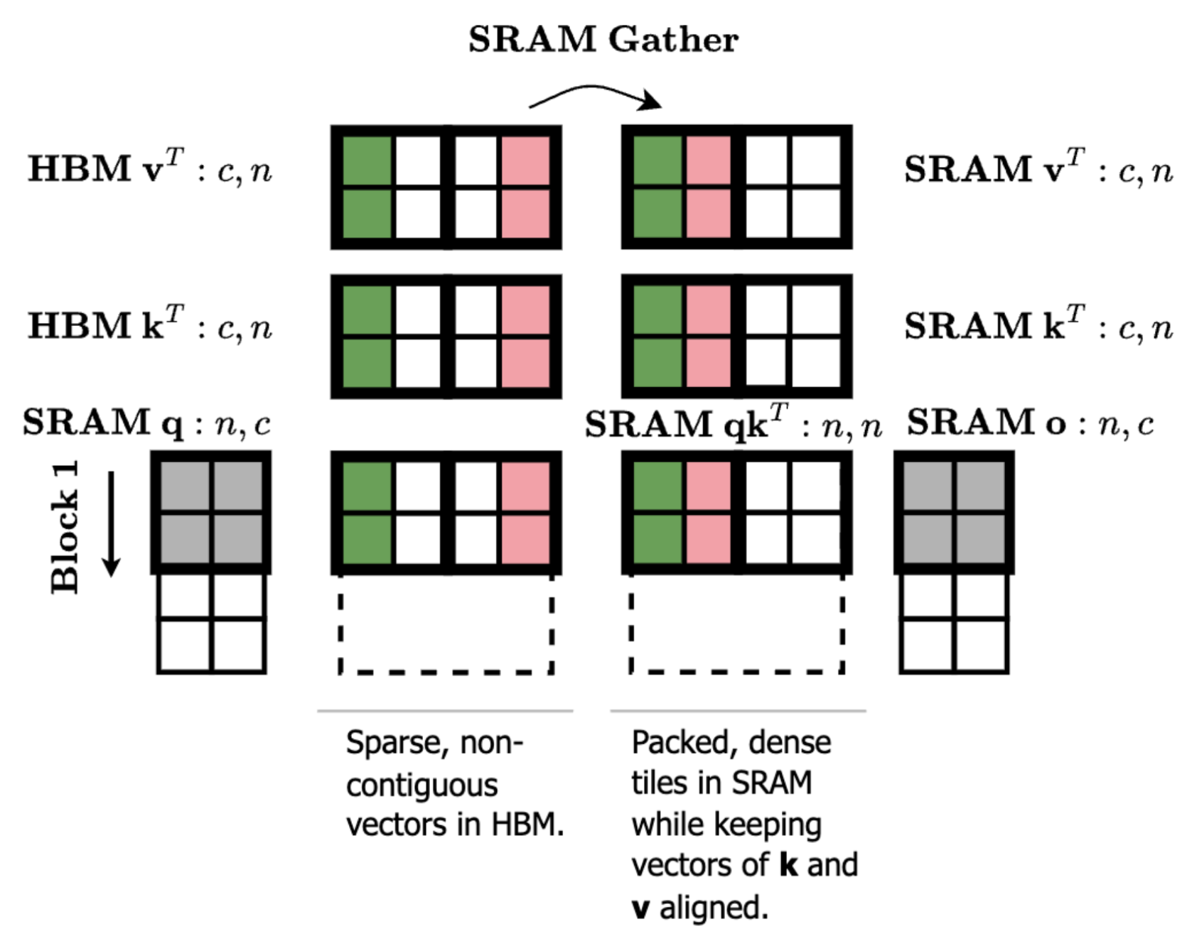
The more granular loads incur a small performance penalty, but we find that the sparsity levels make up for this–e.g. at 93% sparsity, our column-sparse attention kernel in ThunderKittens is ~10x times faster than the dense baseline.

Ok, so now we’re working with [128, 1] column sparsity, which corresponds to 128 contiguous tokens recomputing the same set of individual output vectors across steps (atomic latent space movements). Intuitively, we expect that small 2D patches of an image have similar color and brightness. And in video, we expect the same for small 3D cubes (voxels). Yet, the natural token order is raster order from left to right, top down, and frame zero onwards. To create 128-size chunks with the most similar tokens, we reorder the tokens (and RoPe embeddings) once at the beginning of the diffusion process such that a chunk in the flattened sequence corresponds to a patch/voxel. These similar tokens, which we expect to interact with similar keys/values, now share the same set of sparse indices because they occupy contiguous rows of the input matrix. At the end of the diffusion process, we then reverse this reordering before decoding to pixel space.

Where does this leave us?

We’re open sourcing all our code! Come play with our chipmunks at https://github.com/sandyresearch/chipmunk, and if you like what you see, give us a ⭐️.

Chipmunks are even happier if they can train!

We’re incredibly excited about the future of hardware-aware sparsity. There is much work to be done to train models to become sparsity-aware and optimize/make learnable recomputation schedules at a per-step, per-layer, and per-token granularity.