Austin Silveria, Soham Govande, Dan Fu | Star on GitHub

In Part I and II of this post, we took a top down perspective to reason about how the diffusion generation process’s movements in latent space can be well-approximated with sparse deltas in attention and MLP computations. In Part III, we’ll look from these granular sparse deltas down to the hardware–how can we maintain peak GPU performance with this sparsity and caching pattern?

Fine-grained sparsity in attention and MLP kernels is challenging due to GPUs being optimized heavily for dense block matrix multiplications. Our column-sparse attention and MLP kernels address this with “tile packing.” We opt for granular loads from global memory to pack a dense shared memory tile to maximize tensor core utilization–with 93% dynamic [192, 1] column sparsity, our sparse ThunderKittens attention kernel is 9.3x faster than the dense baseline.

The use of dynamic sparsity and activation caching brings three more challenges:

1. Identifying the dynamic sparsity pattern must introduce minimal overhead.
2. The extra I/O of reading and writing from the cache should be fast.
3. The cache memory must not exceed the system’s total memory.

To address these, we:

1. Compute indices efficiently with custom top-k, scattering, and fused column-sum attention kernels in CUDA (≥2x faster than PyTorch implementations)
2. Leverage the asynchrony of the cache writeback to allocate streaming multiprocessors (SMs) during future GEMM kernel tail effects (i.e., wave quantization)
3. Build a CPU to GPU pipeline for cache data, overlapping compute/communication, while minimizing memory usage

In the rest of this post, we’ll unpack each of these in detail:

1. GPU Architecture: GPUs love big data loads and big matrix multiplications.
2. Tile Packing: For both attention and MLP, we can pack dense shared memory tiles from non-contiguous columns in global memory.
3. Fast Sparsity Pattern Identification: Fused custom kernels can efficiently identify dynamic sparsity patterns during dense steps.
4. Fast Cache Writeback: The asynchrony of the cache writeback enables us to precisely allocate SMs to this I/O-bound operation.
5. Low Memory Overhead: Activation cache memory can be pipelined from the CPU to minimize our GPU memory footprint.

GPUs = Tensor Cores + Pit Crew

Modern GPUs are extremely optimized for large, block matrix multiplications. Tensor cores (the matrix multiplication unit on Nvidia GPUs) account for essentially all of the FLOPs, and everything not running on tensor cores runs about an order of magnitude (or more) slower.

Let’s start with a brief look at the core hardware components and how they’re designed to keep the tensor cores fully saturated. The authors of ThunderKittens provide a wonderful, in-depth discussion of this in their blog post and paper–we’ll summarize here.

GPUs are made up of many independent streaming multiprocessors (e.g., 132 SMs on an H100), each with their own compute units and fast local memory (SRAM). Global memory, or High-Bandwidth Memory (HBM), is slower than SRAM and shared among all SMs. A typical dataflow in kernels (programs that run on GPUs) looks like the following:

1. Load a big tile (block) of data from HBM to SRAM
2. Feed two tiles of data from SRAM to the tensor cores
3. Store the matrix multiplication output in SRAM
4. Fuse other operations while data is in SRAM (e.g. softmax, GeLU, bias)
5. Store the final results in HBM

The most critical path in this dataflow is feeding the tensor core. If the tensor core is not fully saturated, the kernel is losing significant FLOP utilization.

On H100s, there are two key hardware abstractions that contribute the most to tensor core utilization: Tensor Memory Accelerator (TMA) and Warp-Group Matrix Multiply Accumulate instructions (WGMMAs).

To see why we need TMA and WGMMAs, let’s walk through FlashAttention-3 (FA3) at a high level. FA3 partitions work across the H100’s 132 Streaming Multiprocessors (SMs) as chunks of rows in the intermediate [n, n] attention matrix. Each SM loads a chunk of queries from global to shared memory and slides right across this intermediate matrix as it incrementally loads chunks of key and values to compute the attention output. With more query chunks than SMs, each SM has an outer loop over chunks.

We use TMA for global to shared loads/stores, and WGMMAs for big matrix multiplications:

1. Load a big, dense 2D tensor from HBM to dense 2D SRAM with TMA
2. Swizzle on the way from HBM to shared memory with TMA (more on this in a second)
3. Split TMA loads and WGMMA compute between producer/consumer specialized warp groups
4. Store to HBM with TMA

So, four questions:

1. Why do we need to load big, dense blocks with TMA?
2. What is swizzling and why do we need it?
3. Why do we need WGMMAs?
4. Why do we need to warp-specialize for TMA loads/WGMMAs?

(1) Generating global/shared memory addresses for a lot of granular data loads is expensive. The tensor cores are so fast that doing the arithmetic for address generation and issuing a large number of granular load instructions becomes a bottleneck. TMA is a dedicated hardware unit that relieves this pressure–it loads a dense multidimensional tensor from HBM to shared memory with a single instruction and writes to shared memory in a swizzled layout.

(2) Swizzling reorders data in shared memory for fast loads to registers. Two notes on shared memory: (i) shared memory has 32 physical “banks”, and (ii) accesses to different memory in the same bank are serialized (“bank conflicts”). For the fastest shared memory accesses by our WGMMAs, we need to eliminate bank conflicts. That is, parallel shared memory accesses across threads need to be evenly distributed across banks. Swizzling does this by reordering the data in shared memory according to statically defined patterns.

(3) Only warpgroup-level MMAs can saturate the tensor core. Warps are groups of 32 threads executing on the same SM and 4 warps make up a warp group. Warp-level MMAs only go up to 16x16x16, whereas warp-group MMAs (WGMMAs) go up to 64x256x16. The bigger, the better.

(4) Producer/consumer warp-specialization can improve register usage. Even though the H100’s TMA loads and WGMMAs are already asynchronous, having separate warps enables consumers to take on more registers, useful for our register-hungry WGMMAs!

The main takeaway from this discussion of GPU hardware is that to make our kernels fast, we should aim to fully saturate the tensor cores with large block matrix multiplications at all times. TMA, swizzling, and warp-specialization are all techniques that let us get data to the tensor cores faster, in the format they want.

But fine-grained sparsity goes against this. The purpose of granular sparsity is to skip the unimportant pieces of computation to get an end-to-end wall clock speedup. But if we have finer granularity than the large tensor core matrix multiplication sizes, then our tensor cores won’t be saturated, and we won’t realize the full theoretical speedup.

So to write efficient sparse kernels, we must answer the following question: How can we compute granular sparsity patterns with dense, block matrix multiplications?

Tile Packing: Efficient Column Sparse Attention and MLPs

To move toward expressing sparse attention and MLPs with dense, block matrix multiplications, let’s unpack what attention and MLPs are actually computing.

Starting with the equations, we have:

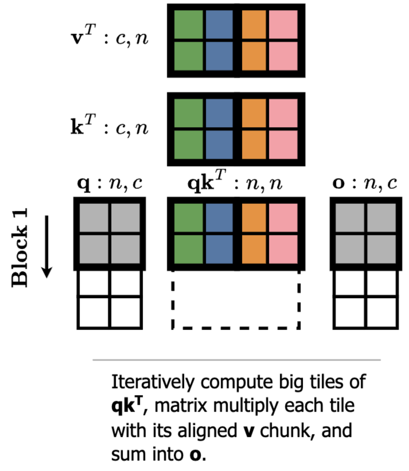
1. Attention: softmax(Q @ KT) @ V
2. MLP: gelu(X @ W1) @ W2

Both operations compute a query/key/value operation with a non-linearity applied to the query-key product. In attention, the key/value vectors are dynamic (projected from the current token representation). In MLP, the key/value vectors are static (columns of the weights W1, and rows of W2).

And as we’ve seen, GPUs like to compute large blocks of the intermediate matrix at once (the query-key scores).

So if we compute with block sparsity that aligns with the native tile sizes of the kernel, it is essentially free because the tensor cores get to use the same large matrix multiplication sizes and skip full blocks of work. But finer granularity presents a problem because we’d have sparsity patterns that don’t align with the large tensor core block sizes, leading to low utilization.

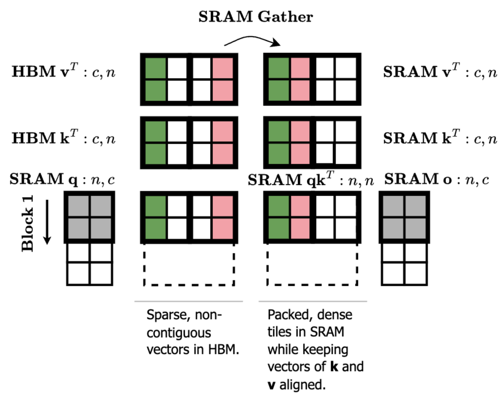
However, there is one optimization we can make to efficiently get to column sparsity in the intermediate matrix. Looking at our matrix multiplication diagram, let’s think through what happens if we reorder the columns of kT and vT. A reordering of kT will apply the same reordering to the columns of A = q @ kT. And if we apply the same reordering to vT, then the end result o is actually the same because the columns of A still align with the correct columns of vT.

What this allows us to do is compute attention or MLP with any ordering of the keys/values in shared memory–thus for [192, 1] sparsity, we can maintain the native compute tile sizes of [192, 128] and pack our sparse keys/values from non-contiguous rows in global memory into a dense tile in shared memory. As a result, our fast kernels can take on any static sparsity pattern (e.g. sliding tile attention) by just passing in a particular set of indices to attend to.

But wait, didn’t we say we needed to load large blocks from HBM to SRAM with TMA to avoid bottlenecking the tensor cores?

While TMA is necessary to achieve peak performance, we find that using granular 16 byte cp.async loads still retains 85-90% of performance in the dense kernel. And with 93% dynamic [192, 1] sparsity in our kernel at HunyuanVideo shapes (sequence length 118k, head dim 128, non-causal), we see a 9.3x speedup over the dense TMA baseline (65% of theoretical speedup).

Our first set of optimizations was guided by the fact that our MLP epilogues are expensive operations. Since the MLP value vectors are rows of the static weight matrix W2, the computation of cross-step MLP deltas can be computed in one shot. We cache the previous step post-nonlinearity activations and output and directly compute a delta of this output cache: We (1) compute the delta of our current step’s sparse activations and the cache, (2) multiply this sparse delta with the value-vectors (rows of W2), and (3) add this output directly to the output cache.

This brings challenges for the epilogue of the first matrix multiplication: We add a bias, apply GeLU, scatter the results into the unpacked activation cache global memory, subtract the post-activation cache, and store to global memory. This takes valuable time away from tensor core activity.

But we can fix this with a persistent grid + warp-specialized kernel! The producer warpgroup’s prologue can overlap with the consumer warpgroups’ epilogue if multiple work tiles are mapped to a persistent threadblock. This means that while the consumer is cranking away at low-utilization operations, the producer can queue up the next memory load instructions. Persistent grids aren’t new—but they made an especially big impact on an epilogue-heavy kernel like this.

Fast Identification of Dynamic Sparsity Patterns

So, we’ve found that [192, 1] sparsity on the intermediate activation matrix can be efficient, but we still have the issue of dynamically identifying the most important columns with minimal overhead.

In training-aware sparsity, there is the option of letting the model learn to directly select the sparsity patterns. For training-free sparsity, however, we need to compute a heuristic from the activations to determine the most important sparse subset of our computation. In Diffusion Transformers (DiTs), we can do this efficiently by exploiting the fact that activations change slowly across steps (see Part II for more detail on DiTs and their activation distributions).

Our sparse attention delta algorithm (i) identifies important [192, 1] columns during a small set of dense steps, and then (ii) reuses these indices for a number of subsequent sparse steps. Within the dense attention kernel, we’d ideally be able to fuse a column sum directly after the q @ kT multiplication, but this would be a column sum over the unnormalized logits which results in uneven scales across rows. And even if we switched to fusing a column sum after the softmax in the dense kernel, this would result in each tile having different scales since FlashAttention computes the softmax incrementally over the tiles.

We find that a simple trick solves this problem: Reuse the softmax constants from a previous step to compute the column sums. Since the activations change slowly across steps, the old softmax constants are still a good normalization of the logits that can be applied to all tiles before the column sum.

This fused kernel outputs the normal dense attention output (computed using the correct softmax constants) and a column sum (computed with the reused softmax constants) that we can pass to a TopK operation.

But, we noticed that at smaller sequence lengths, torch.topk was introducing significant overhead relative to the total time of our MLP GEMMs. We can do better! We wrote a fast approximate top-k kernel that uses CUDA shared memory atomics and quantile estimation to beat PyTorch by 2x (and when we compute these indices, our custom cache writeback kernel (1.5x faster than PyTorch), can process them).

Fast Cache Writeback

The longest stage of the first MLP GEMM epilogue was scattering the results into unpacked activation cache global memory. What if we could fuse this memory-bound scatter-add operation into the next compute-bound GEMM? We were eager to find out!

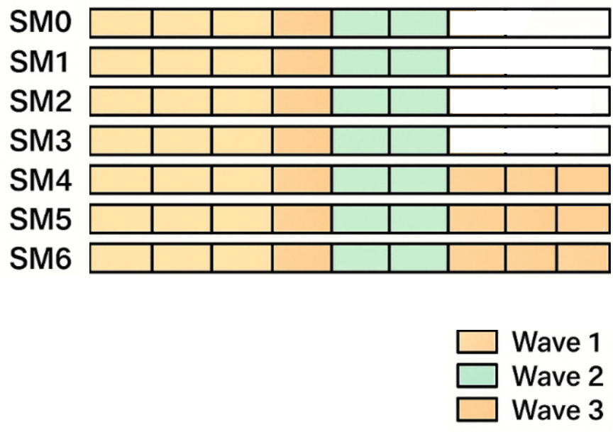
We wrote some code using CUDA driver API to allocate a handful of streaming multiprocessors (SMs) to a custom kernel implementing the cache writeback operation, while using the rest of the SMs for the GEMM. Since nearly every GEMM suffers from some degree of wave quantization, this does not impact the runtime of the GEMM—it just repurposes any leftover compute. Our custom cache writeback kernel uses the latest TMA-based reduction PTX instructions (cp.reduce.async.bulk) to perform large atomic updates into global tensors (3x faster than naive in-register reductions), and this lets us save ~20 microseconds on every MLP invocation!

Minimize Memory Overhead

What about managing cache memory? Since we’re computing sparse deltas against cached per-layer activations and reusing per-layer sparse indices across steps, how much memory does this consume?

On a single GPU at a sequence length of 118k, a lot!

Each layer has (i) a boolean mask to mark the active [192, 1] columns of the intermediate attention matrix and (ii) a cache of the previous step’s attention output. But with two optimizations we can significantly reduce this memory pressure:

1. Bitpack the sparsity mask (since torch.bool is 1 byte per value by default)
2. Offload the masks and activation cache to CPU memory with overlapped compute/communication

	Naive	Optimized	Memory Reduction
Sparsity Mask Cache	104 GB	430 MB	242x
Activation Cache	43 GB	1.4 GB	31x

We find that a simple torch compiled bitpack function gives us a quick 8x memory reduction on the sparsity mask with very small overhead.

And for offloading, PCIE-5’s 64 GB/s is not slow! We preallocate pinned tensors (page locked) in CPU memory and double buffer in GPU memory so we can load the next layer’s mask and activation cache during the computation of the current layer.

Where does this leave us?

We’re big fans of ThunderKittens, and so are our chipmunks! Our sparse attention and MLP kernels let our chipmunks play nicely with their kitten friends.

In the last few sections, we’ve made progress toward more efficient fine-grained dynamic sparsity in attention and MLPs and highlighted an application of computing training-free cross-step sparse deltas in DiTs.

Beyond what we’ve already done, there are a few more optimizations that pique our interest. Even though we can potentially load 256 contiguous bytes from global (2-byte BF16 * head dim 128), we’re using 16 byte cp.async instructions to align with the default 16-byte atomicity of the 128-byte swizzling (16-byte chunks of data are kept intact while swizzling). But, we may be able to use larger loads by trading a small amount of sparsity granularity. Since the 128-byte swizzle pattern repeats every 1024 bytes, we could use a [192, 4] sparsity pattern that loads 4 contiguous keys/values (1024 contiguous bytes from global) using a single TMA load instruction that handles swizzling. A couple more fun possibilities are trying to do packing on the way from SRAM to registers, using the ldmatrix instruction (as “consecutive instances of row need not be stored contiguously in memory”), or working with the new column mask descriptor on the Blackwell tcgen05.mma instruction.

Overall, we think there’s a lot of unexplored territory around granular dynamic sparsity in kernels. We’re excited to further explore training-aware attention sparsity, optimize for even finer granularity, and integrate sparse deltas with more model architectures.

And we’re open sourcing everything! Check out our repo at https://github.com/sandyresearch/chipmunk and come hack on kernels with chipmunks!